The 2D case is identified here as the waveguide with cylindrical symmetry discussed in
section 2.2.3,
so the coordinates  ,
,  and
and  stand for horizontal distance,
depth and ray slope related to the horizontal,
respectively.
The Gaussian beam expression for this case follows readily from the expression for the 2.5 case,
by taking
stand for horizontal distance,
depth and ray slope related to the horizontal,
respectively.
The Gaussian beam expression for this case follows readily from the expression for the 2.5 case,
by taking  and
and  ,
which provides the expression
,
which provides the expression
![\begin{displaymath}
P(s,n) = \frac {1}{4\pi}\sqrt{ \frac {c(s)}{c(0)} \frac {\co...
...au(s) + \frac{1}{2}\frac {p(s)}{q(s)} n^2 \right) \right] ;
\end{displaymath}](img150.png) |
(3.7) |
in this expression  and
and  are related through the so-called dynamic equations:
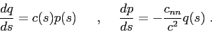 |
(3.8) |
The second-order derivative along the normal can be written in terms of derivatives along and
as[1]
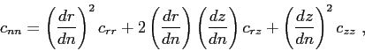 |
(3.9) |
where
and
Those derivatives can be identified as the components of the polarization vector
 ,
which in the 2D case correspond to:
,
which in the 2D case correspond to:
(see Fig.3.3).
Figure 3.3:
Polarization vectors for the 2D case.
![\includegraphics[height=80mm]{ese1}](ese1.png) |
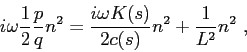
The beam width and curvature,  and
and  , respectively[1,9],
can be calculated from and by comparing the following expressions:
, respectively[1,9],
can be calculated from and by comparing the following expressions:
which yields that
![\begin{displaymath}
K(s) = c(s) \makebox{Re}\left[ \frac {p(s)}{q(s)} \right] ,
\end{displaymath}](img163.png) |
(3.10) |
and
![\begin{displaymath}
L(s) = \sqrt{ \frac {-2}{\omega \displaystyle { \makebox{Re}\left[ \frac {p(s)}{q(s)} \right] }} } .
\end{displaymath}](img164.png) |
(3.11) |
As shown by Eq.(3.11) the Gaussian beam approximation requires that 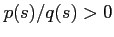 .
To this end it would be sufficient to select a non-zero real value for
.
To this end it would be sufficient to select a non-zero real value for  ,
plus the choice
,
plus the choice
 ,
being
,
being  a real number,
as small as possible.
Orlando Camargo Rodríguez
2012-06-21
a real number,
as small as possible.
Orlando Camargo Rodríguez
2012-06-21
![\begin{displaymath}
\mbox{$\mathbf{e}$}_s(s) =
\left[
\begin{array}{c}
\cos\th...
...ay}{r}
-\sin\theta(s) \\
\cos\theta(s)
\end{array} \right]
\end{displaymath}](img158.png)