Near source fields

The examples of the previous sections used Bellhop's default option to calculate acoustic pressure, namely, geometric beams, which sometimes can be not sufficiently accurate for particular applications. To this effect Bellhop provides additional approximations to improve accuracy. Let us illustrate this through the calculation of coherent transmission loss near the source with different approximations, so the interference pattern reveals the accuracy of the approximation used. First, we copy flatwav.env to nearsource.env, which now looks like follows:

'Munk profile/Near source field'
50.0			
1			
'SVF'			
51  0.0  5000.0
    0.0  1548.52  /
  200.0  1530.29  /
  250.0  1526.69  /
  400.0  1517.78  /
  600.0  1509.49  /
  800.0  1504.30  /
 1000.0  1501.38  /
 1200.0  1500.14  /
 1400.0  1500.12  /
 1600.0  1501.02  /
 1800.0  1502.57  /
 2000.0  1504.62  /
 2200.0  1507.02  /
 2400.0  1509.69  /
 2600.0  1512.55  /
 2800.0  1515.56  /
 3000.0  1518.67  /
 3200.0  1521.85  /
 3400.0  1525.10  /
 3600.0  1528.38  /
 3800.0  1531.70  /
 4000.0  1535.04  /
 4200.0  1538.39  /
 4400.0  1541.76  /
 4600.0  1545.14  /
 4800.0  1548.52  /
 5000.0  1551.91  /
'A'  0.0
 5000.0  1600.00 0.0 1.8 .8 /
1
  1000.0 /		
501
    0.0 2000.0 /	
501
  0.2  10.0 /	
'C'
201
 -25.0 25.0  /       
0.0  5500.0  102.0,
'MS' 1.0  100.0 0,
3  5

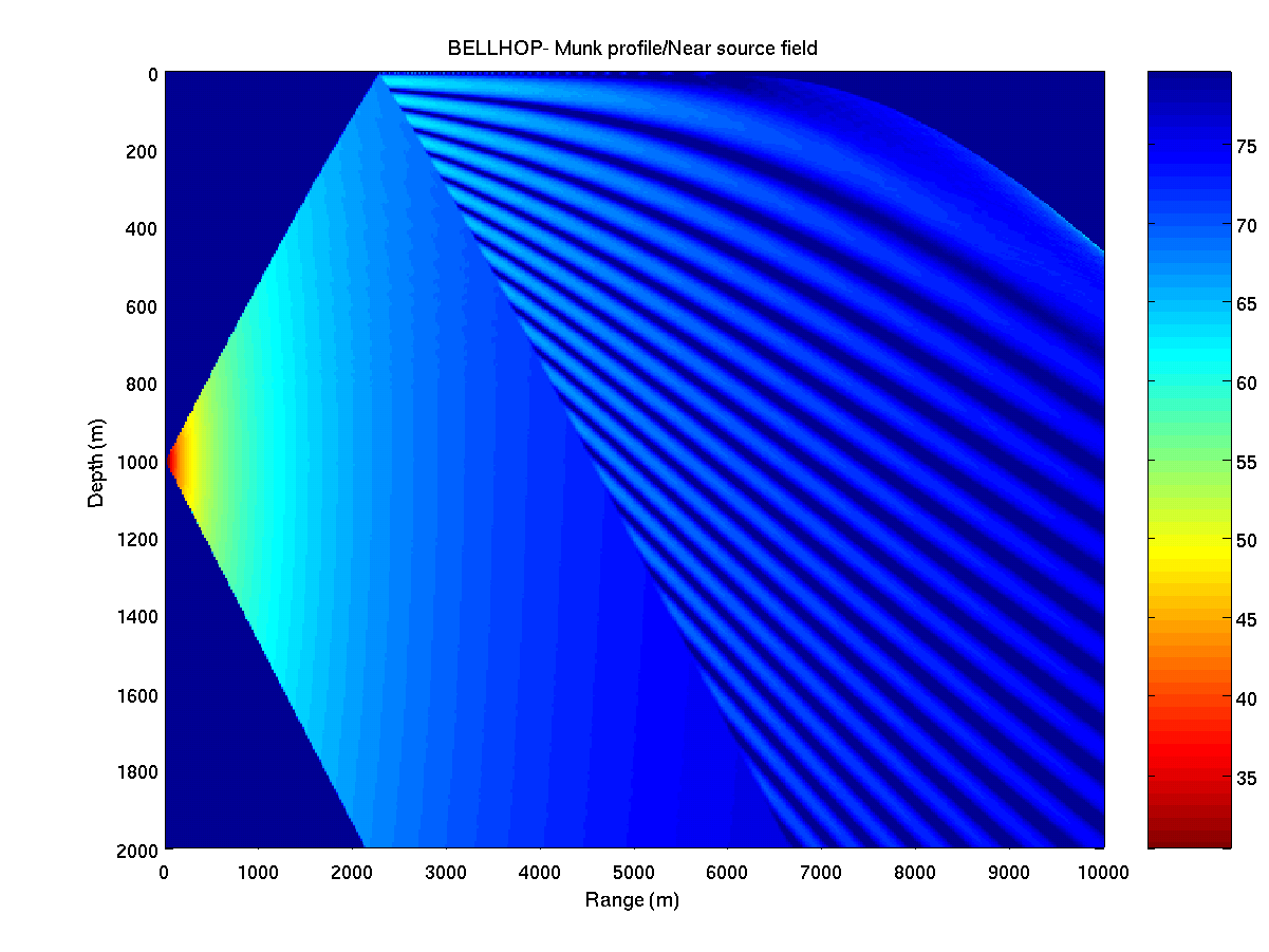
We can notice the inclusion of two additional lines (in fact, the beam block). When using geometric beams, by setting OPTIONS3(1) = 'C', those lines are ignored, but we are including them in advance in order to make automatic the transition to the other approximations. Running Bellhop with nearsource.env allows us to obtain Fig.8. As shown by the figure the acoustic field is strictly confined between the propagating rays and the interference pattern of acoustic pressure becomes visible only at a large distance from the source. Similar results will be obtained using Gaussian beam bundles, when we change OPTIONS3(1) = 'C' to OPTIONS3(1:2) = 'CB' in nearsource.env.

Figure 8: Coherent transmission loss calculated by Bellhop near the source using geometric beams.

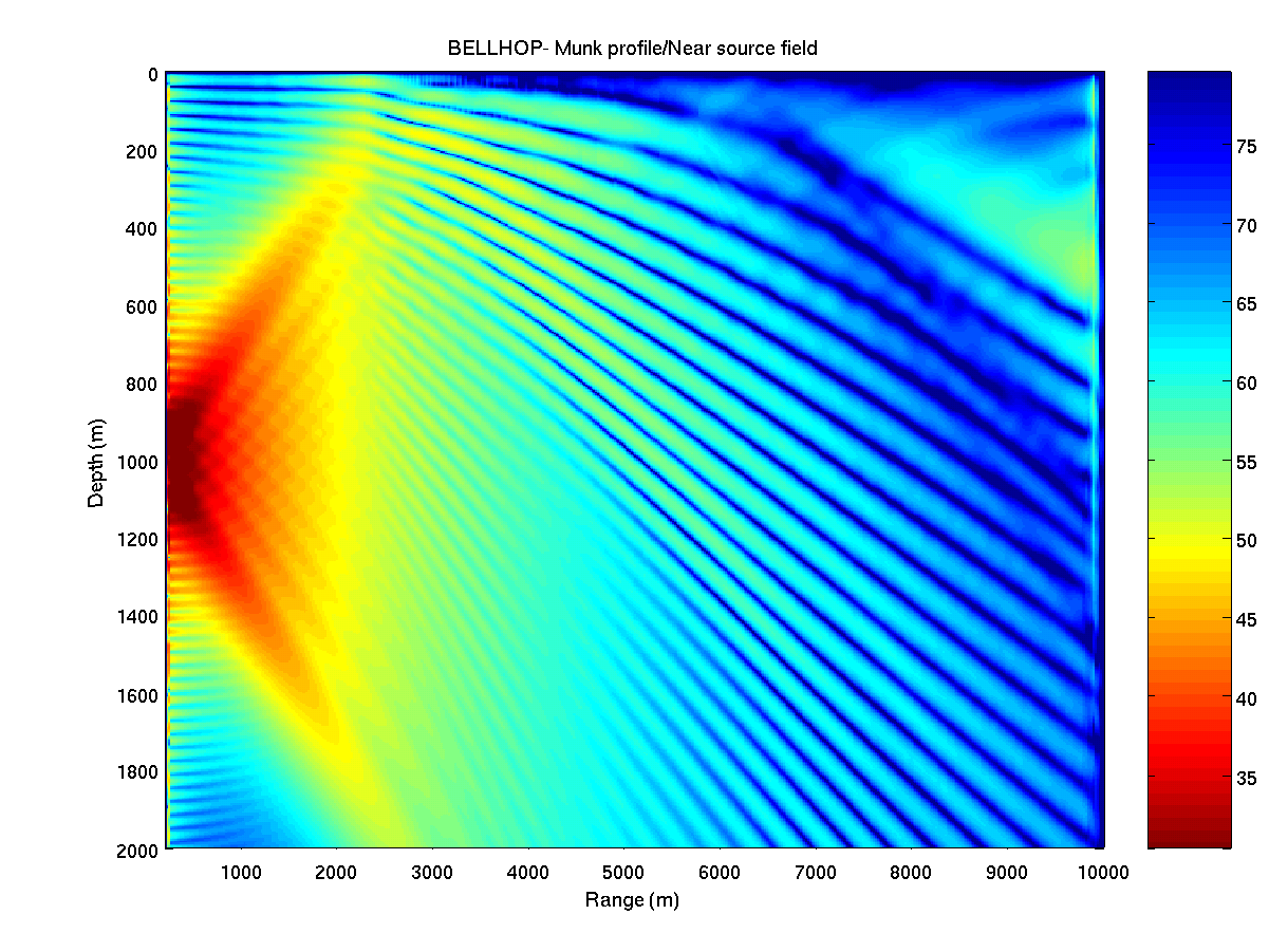
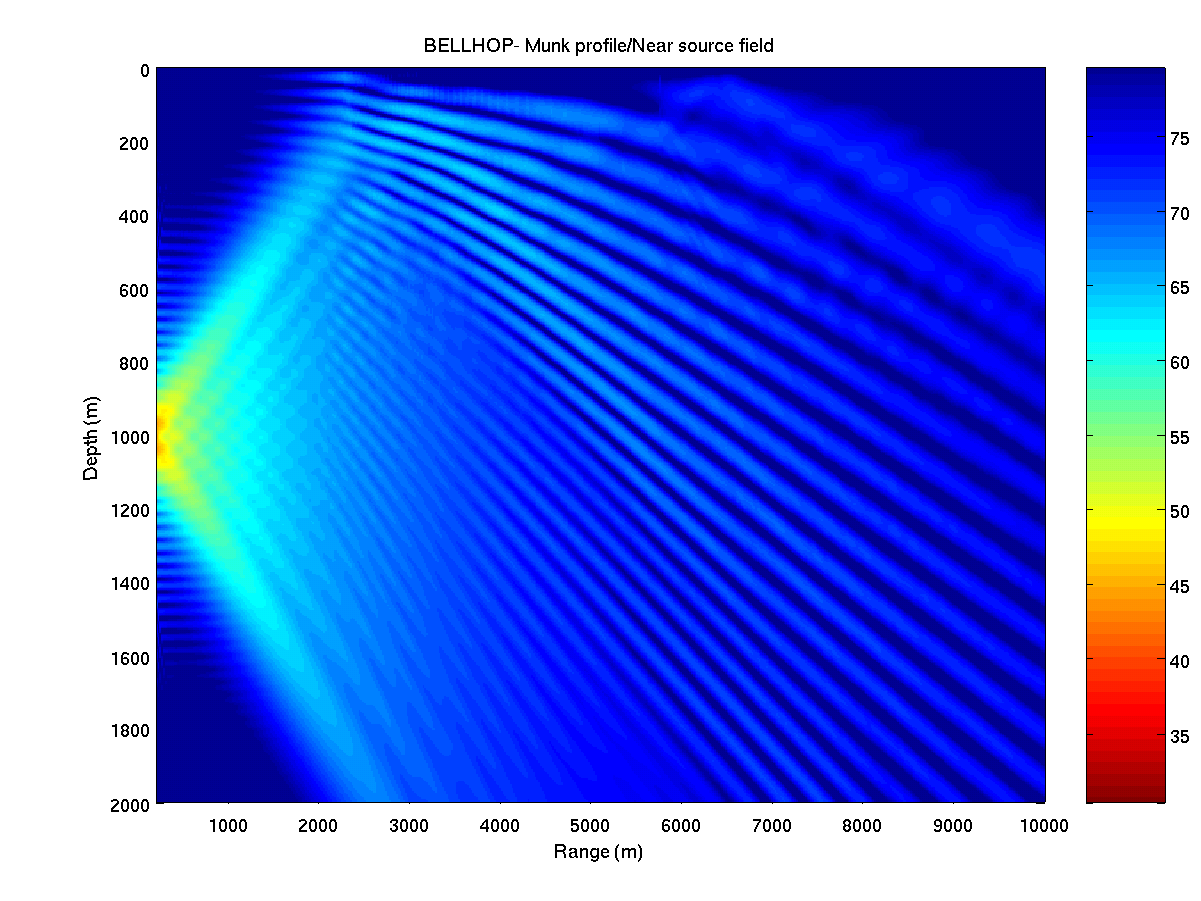
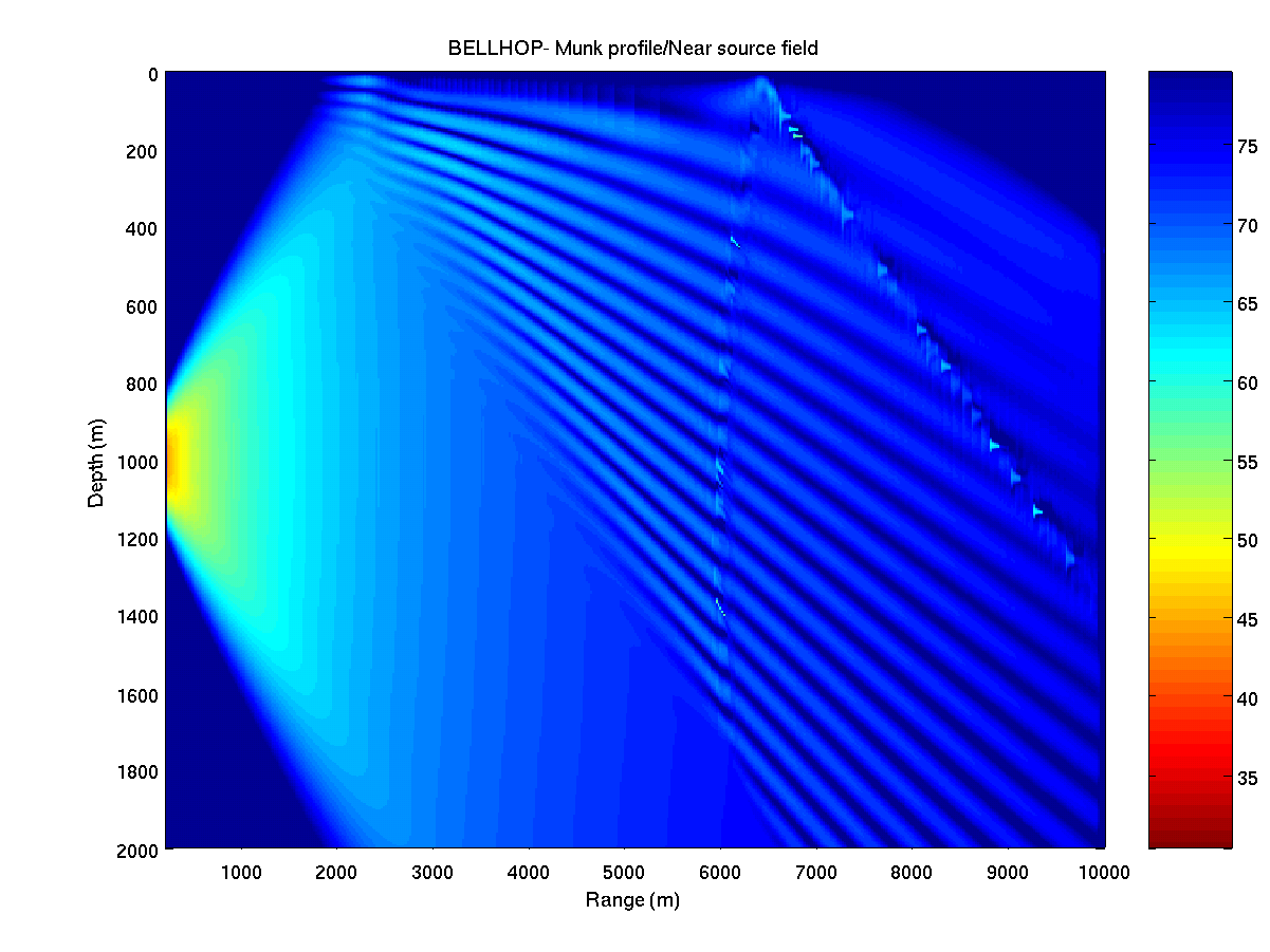
A completely different pattern is revealed when we switch on the calculation of beams influence using Cartesian coordinates, by setting OPTIONS3(1:2) = 'CC' and OPTIONS4(1:2) = 'MS'. As shown in Fig.9 the acoustic field reveals an accurate pattern of interference, which now spans over the entire watercolumn. A similar result, although with minor differences in amplitude, can be obtained using ray centered coordinates (OPTIONS3(1:2) = 'CR', see Fig.10). However, the structure of the pattern depends on the type of beam curvature. For instance, setting OPTIONS4(1:2) = 'CZ' will lead us to Fig.11.

Figure 9: Coherent transmission loss calculated by Bellhop near the source using Cartesian coordinates to calculate the beams influence. Beam type is 'MS'.

Figure 10: Coherent transmission loss calculated by Bellhop near the source using ray centered coordinates to calculate the beams influence. Beam type is 'MS'.

Figure 11: Coherent transmission loss calculated by Bellhop near the source using Cartesian coordinates to calculate the beams influence. Beam type is 'CZ'.