A flat waveguide

Let us start with a simple ray trace between 0 and 101 km, using an input file called flatwav.env. The file looks like this:

'Munk profile/Flat waveguide' 
50.0
1
'SVW'
51  0.0  5000.0	
    0.0  1548.52  /
  200.0  1530.29  /
  250.0  1526.69  /
  400.0  1517.78  /
  600.0  1509.49  /
  800.0  1504.30  /
 1000.0  1501.38  /
 1200.0  1500.14  /
 1400.0  1500.12  /
 1600.0  1501.02  /
 1800.0  1502.57  /
 2000.0  1504.62  /
 2200.0  1507.02  /
 2400.0  1509.69  /
 2600.0  1512.55  /
 2800.0  1515.56  /
 3000.0  1518.67  /
 3200.0  1521.85  /
 3400.0  1525.10  /
 3600.0  1528.38  /
 3800.0  1531.70  /
 4000.0  1535.04  /
 4200.0  1538.39  /
 4400.0  1541.76  /
 4600.0  1545.14  /
 4800.0  1548.52  /
 5000.0  1551.91  /
'A'  0.0
 5000.0  1600.00 0.0 1.8 .8 
1
1000.0 /
1
1000.0 /
1
101.0 /
'R'
70
 -13.0 13.0  /
100.0  5500.0  102.0

On the command line one invokes Bellhop by writing

whatevershell$ bellhop flatwav <ENTER>

Once Bellhop finishes with calculations one can verify that two files were created: the first is called flatwav.prt, with general information regarding the waveguide characteristics, number of launching angles, calculation time, etc, etc. The second one is called flatwav.ray, and it is an ASCII file containing ray coordinates. One can plot them using the M-file plotray.m:

>> plotray( 'flatwav' ) <ENTER>

which generates Fig.1. Changing OPTIONS3(1) = 'R' to OPTIONS3(1) = 'E' and proceeding as before one can obtain the eigenrays shown in Fig.2.

Figure 2: Rays calculated by Bellhop in a flat deep water waveguide.

Figure 3: Eigenrays calculated by Bellhop in a flat deep water waveguide.

The calculation of coherent transmission loss requires some minor modifications to the input file. First, we set OPTIONS3(1) = 'C'; second, let us consider that transmission loss will be calculated on a rectangular grid with 501$\times$501 points in range and depth. Finally, let us let set nbeams = 0 and let Bellhop decide how many rays are required. The input file then becomes:

'Munk profile/Flat waveguide'
50.0
1
'SVW'
51  0.0  5000.0
    0.0  1548.52  /
  200.0  1530.29  /
  250.0  1526.69  /
  400.0  1517.78  /
  600.0  1509.49  /
  800.0  1504.30  /
 1000.0  1501.38  /
 1200.0  1500.14  /
 1400.0  1500.12  /
 1600.0  1501.02  /
 1800.0  1502.57  /
 2000.0  1504.62  /
 2200.0  1507.02  /
 2400.0  1509.69  /
 2600.0  1512.55  /
 2800.0  1515.56  /
 3000.0  1518.67  /
 3200.0  1521.85  /
 3400.0  1525.10  /
 3600.0  1528.38  /
 3800.0  1531.70  /
 4000.0  1535.04  /
 4200.0  1538.39  /
 4400.0  1541.76  /
 4600.0  1545.14  /
 4800.0  1548.52  /
 5000.0  1551.91  /
'A'  0.0
 5000.0  1600.00 0.0 1.8 .0 /
1
  1000.0 /
 501
   0.0 5000.0 /	
 501
    0.0 101.0 /	
'C'
0
 -14.0 14.0  /          
100.0  5500.0  102.0

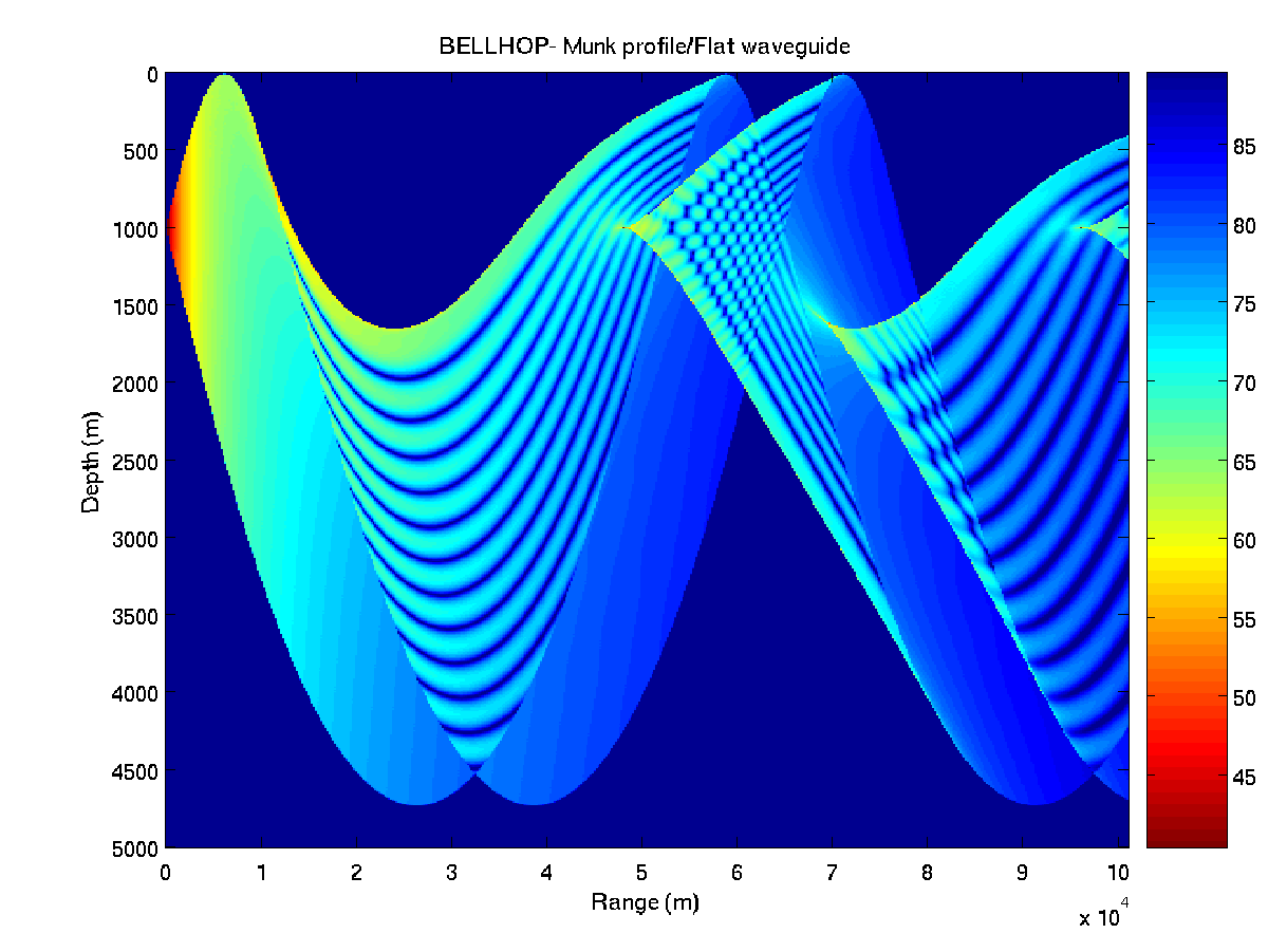
Now, after running Bellhop one obtains a binary file called flatwav.shd, which in fact contains the acoustic pressure, calculated coherently. We can plot the transmission loss using the M-file plotshd.m:

>> plotshd( 'flatwav.shd' ) <ENTER>

which produces Fig.4.

Figure 4: Coherent transmission loss calculated by Bellhop.

Finally, let us set OPTIONS3(1) = 'A' and modify flatwav.env as shown bellow:

'Munk profile/Flat waveguide'
50.0			
1			
'SVW'			
51  0.0  5000.0
    0.0  1548.52  /
  200.0  1530.29  /
  250.0  1526.69  /
  400.0  1517.78  /
  600.0  1509.49  /
  800.0  1504.30  /
 1000.0  1501.38  /
 1200.0  1500.14  /
 1400.0  1500.12  /
 1600.0  1501.02  /
 1800.0  1502.57  /
 2000.0  1504.62  /
 2200.0  1507.02  /
 2400.0  1509.69  /
 2600.0  1512.55  /
 2800.0  1515.56  /
 3000.0  1518.67  /
 3200.0  1521.85  /
 3400.0  1525.10  /
 3600.0  1528.38  /
 3800.0  1531.70  /
 4000.0  1535.04  /
 4200.0  1538.39  /
 4400.0  1541.76  /
 4600.0  1545.14  /
 4800.0  1548.52  /
 5000.0  1551.91  /
'A'  0.0
 5000.0  1600.00 0.0 1.8 .0 /
1
  1000.0 /
 1
   1000.0 /
 1
    101.0 /
'A'
101
 -14.0 14.0  /
100.0  5500.0  102.0

After running Bellhop one obtains an ascii file called flatwav.arr, with the amplitudes and travel times of the rays that arrive at the receiver position (we indicated only one, but the model is able to calculate travel times and amplitudes at all points of the array indicated in the array block). The data contained in the *.arr file can be read using the M-file read_arrivals_asc.m:

>>  [ a, tau, theta0, thetaR, srefl, brefl, narr, rz ] = ... 
read_arrivals_asc( 'flatwav.arr' ) <ENTER>