The input file

The general structure of the input file (hereafter WAVFIL) can be better understood if one thinks of it as composed of blocks, with each block describing a particular element of the waveguide, from top to bottom. In order to provide a visually friendly structure of the WAVFIL the blocks are separated with a line, which is ignored by the model. The structure of the WAVFIL is as follows:

Title
Source	Block
Altimetry	Block
Sound Speed	Block
Object	Block	(Traceo only)
Bathymetry	Block
Output	Block

The Title is a character string, which is written in both the LOGFIL (the file with the *.log extension) and the OUTFIL (the output file).

The structure of each block is as follows:

Source Block:

ds	ray step
rs	source range coordinate
zs	source depth coordinate
cs	sound speed at the source position
freqs	source frequency
bmtype	beam type
nthtas	number of launching angles
thetas(1) thetas(nthtas)	first and last launching angles

At the present moment bmtype can be set only to 'GMB' (Geometric Gaussian Beams), future versions of the models will include other types of Gaussian beams.

Altimetry Block:

inttype	interpolation type ('2P'/'3P')
stype	surface type ('V', for vacuum/'R', for rigid)
n	number of surface coordinates
rati(1) zati(1)	surface coordinates
rati(2) zati(2)
rati(3) zati(3)
...
rati(n) zati(n)

With inttype = '3P' the model performs parabolic interpolation around the interpolation point; with inttype = '2P' simpler linear interpolation is used. The maximal value of surface range (rati(n)) is taken as maximal range. Sound speed is not interpolated above surface values.

Sound Speed Block:

ctype	type of sound speed distribution
ptype	particular type of sound speed

ctype can correspond to

'c(z,z)'	sound speed profile	$c = c(z)$,
'c(r,z)'	sound speed field	$c = c(r,z)$.

For a sound speed profile range derivatives are zero and depth derivatives are calculated depending of the type of the profile (defined by ptype). For a sound speed field both range and depth derivatives are calculated using a bi-dimensional parabolic interpolation. At present such fields can be defined only on a rectangular grid.

When ctype = 'c(z,z)' the parameter ptype allows to define a set of analytical profiles (so both sound speed and its derivatives are calculated analytically at the interpolation point) or a numerical profile. For any of the analytical profiles the Sound Speed Block should be defined as:

n	number of depths (ignored)
z(1) c(1)	sound speed data
z(2) c(2)

With the exception of the isovelocity profile the depths and sound speeds are required to be different (otherwise the program produces a warning and stops). For the analytical profiles the parameter ptype can take one of the following values:

1. 'ISOV' (isovelocity profile):
   
   $$c(z) = c_0 = \makebox{ constant } , \frac{dc}{dz} = 0 , \frac{d^2c}{dz^2} = 0 ,$$
   
   
   where $c_0$ = c(1). The remaining information is ignored.
2. 'LINP' (linear profile):
   
   $$c(z) = c_0 + k\left( z - z_0 \right) , \frac{dc}{dz} = k , \frac{d^2c}{dz^2} = 0 ,$$
   
   
   where $z_0$ = z(1) and $c_0$ = c(1). The constant $k$ is calculated as
   
   $$k = \frac {\makebox{\texttt{c(2)-c(1)}}}{\makebox{\texttt{z(2)-z(1)}}} .$$
   
   

3. 'PARP' (parabolic profile):
   
   $$c(z) = c_0 + k\left( z - z_0 \right) ^2 , \frac{dc}{dz} = 2k\left( z - z_0 \right) , \frac{d^2c}{dz^2} = 2k ,$$
   
   
   where $z_0$ = z(1) and $c_0$ = c(1). The constant $k$ is calculated as
   
   $$k = \frac {\makebox{\texttt{c(2)-c(1)}}}{ \left( \makebox{\texttt{z(2)-z(1)}} \right) ^2 } .$$
   
   

4. 'EXPP' (exponential profile):
   
   $$c(z) = c_0 e^{ -k\left( z - z_0 \right) } ,$$
   
   
   
   
   $$\frac{dc}{dz} = -kc_0 e^{ -k\left( z - z_0 \right) } , \frac{d^2c}{dz^2} = k^2c_0 e^{ -k\left( z - z_0 \right) } ,$$
   
   
   where $z_0$ = z(1) and $c_0$ = c(1). The constant $k$ is calculated as
   
   $$k = \frac {1}{ \makebox{\texttt{z(2)-z(1)}} }\ln\left[ \frac ... ...ebox{\texttt{c(1)}} }{ \makebox{ \texttt{c(2)} } } \right] .$$
   
   

5. 'N2LP' ($n^2$-linear profile):
   
   $$c(z) = \frac {c_0}{ \left[ 1 + k\left( z - z_0 \right) \right] ^{1/2} } ,$$
   
   
   
   
   $$\frac{dc}{dz} = \frac {-kc_0}{2\left[ 1+k\left( z-z_0 \right)... ... {3k^2c_0}{4\left[ 1+k\left( z-z_0 \right) \right] ^{5/2}} ,$$
   
   
   where $z_0$ = z(1) and $c_0$ = c(1). The constant $k$ is calculated as
   
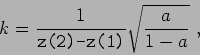
   $$k = \frac {1}{ \makebox{\texttt{z(2)-z(1)}} }\left[ \left( \f... ...tt{c(1)}}}{\makebox{\texttt{c(2)}}} \right) ^2 - 1 \right] .$$
   
   

6. 'ISQP' (inverse-square gradient profile):
   
   $$c(z) = c_0 \left\{ 1 + \frac {k\left( z - z_0 \right) }{ \left[ 1 + k^2\left( z - z_0 \right) ^2 \right] ^{1/2} } \right\} ,$$
   
   
   
   
   $$\frac{dc}{dz} = \frac {kc_0}{2\left[ 1+k^2\left( z-z_0 \righ... ...ht) }{\left[ 1+k^2\left( z-z_0 \right) ^2 \right] ^{5/2}} ,$$
   
   
   where $z_0$ = z(1) and $c_0$ = c(1). The constant $k$ is calculated as
   
   $$k = \frac {1}{ \makebox{\texttt{z(2)-z(1)}} }\sqrt{ \frac {a}{1-a} } ,$$
   
   
   with
   
   $$a = \left[ \frac {\makebox{\texttt{c(1)}}}{\makebox{\texttt{c(2)}}} - 1 \right] ^2 .$$
   
   

7. 'MUNK' (Munk profile):
   
   $$c(z) = c_0 \left[ 1 + \varepsilon( \eta + e^{-\eta} - 1 ) \right] ,$$
   
   
   
   
   $$\frac{dc}{dz} = \frac {2\varepsilon c_1}{B}(1-e^{-\eta}) ,... ...frac{d^2c}{dz^2} = \frac {4\varepsilon c_1}{B^2}e^{-\eta} ,$$
   
   
   with the parameters $\varepsilon = 7,4\times10^{-3}$, $\eta = 2\left( z - z_0 \right) /B$, $B$ = 1,3 km, ($z_0$ represents the depth of the channel axis and $c_0$ the corresponding value of sound speed), where $z_0$ = z(1) and $c_0$ = c(1). The remaining information is ignored.

Finally, the option ptype = 'SSPR' defines an arbitrary sound speed profile, which is defined in the Sound Speed Block as

n	number of depths
z(1) c(1)	sound speed data
z(2) c(2)
z(3) c(3)
...
z(n) c(n)

Depth derivatives are calculated numerically through parabolic interpolation of the sound speed around the interpolation point.

When ctype = 'c(r,z)' the parameter ptype is ignored and the Sound Speed Block continues with the following elements:

m	number of ranges
r(1) r(2) ... r(m)	ranges
n	number of depths
z(1) z(2) ... z(n)	depths
c(1,1) c(1,2) ... c(1,m)	sound speed matrix
c(2,1) c(2,2) ... c(2,m)
c(3,1) c(3,2) ... c(3,m)
...
c(n,1) c(n,2) ... c(n,m)

Range and depth derivatives are calculated numerically through bidimensional parabolic interpolation of the sound speed around the interpolation point.

Object Block (Traceo only):

'H'	(homogeneous object)
inttype	('2P'/'3P')
aunits	(attenuation units)
cobj(1) rhoobj(1) alpha(1)	sound speed, density, attenuation
m	number of object upper coordinates
rup(1) zup(1)	object upper coordinates
rup(2) zup(2)
rup(3) zup(3)
...
rup(m) zup(m)
n	number of object lower coordinates
rdown(1) zdown(1)	object lower coordinates
rdown(2) zdown(2)
rdown(3) zdown(3)
...
rdown(n) zdown(n)

or

'N' (non-homogeneous object)

inttype ('2P'/'3P')

aunits (attenuation units)

m

rup(1) zup(1) cup(1),rhoup(1),alphup(1)

rup(2) zup(2) cup(2),rhoup(2),alphup(2)

rup(3) zup(3) cup(3),rhoup(3),alphup(3)

...

rup(m) zup(m) cup(m),rhoup(m),alphup(m)

n

rdown(1) zdown(1) cdown(1),rhodown(1),alphdown(1)

rdown(2) zdown(2) cdown(2),rhodown(2),alphdown(2)

rdown(3) zdown(3) cdown(3),rhodown(3),alphdown(3)

...

rdown(n) zdown(n) cdown(n),rhodown(n),alphdown(n)

The attenuation units used by both Trace and Traceo models are

'F'	frequency dependent (dB/meter)khz,
'L'	loss parameter,
'M'	dB/meter,
'N'	Nepers/meter,
'Q'	Q-factor,
'W'	dB/wavelength.

For specific details regarding the definitions of these units see [3].

Bathymetry Block:

'H'	bottom type (homogeneous bottom)
inttype	interpolation type ('2P' or '3P')
aunits	(attenuation units)
cbty(1) rhobty(1) alpha(1)	sound speed at bottom, bottom density, attenuation
n	number of bottom coordinates
rbty(1) zbty(1)	bottom coordinates
rbty(2) zbty(2)
rbty(3) zbty(3)
...
rbty(n) zbty(n)

or

'N' bottom type (non-homogeneous bottom)

inttype interpolation type ('2P'/'3P')

n number of bottom coordinates

rbty(1) zbty(1) cbty(1) rhobty(1) alpha(1)

rbty(2) zbty(2) cbty(2) rhobty(2) alpha(2)

rbty(3) zbty(3) cbty(3) rhobty(3) alpha(3)

...

rbty(n) zbty(n) cbty(n) rhobty(n) alpha(n)

The maximal range of bathymetry can not exceed the maximal range of altimetry. Sound speed is not interpolated below bathymetry values.

Output Block:

catype	calculation type
artype	array type

The option catype defines the type of calculations to be performed by the models and the type of information which is going to be written to the OUTFIL; it option can correspond to one of the following:

'RCO'	only ray coordinates;
'ARI'	all ray information;
'EIG'	eigenray information;
'AAD'	only amplitude and delays;
'CPR'	coherent acoustic pressure;
'CTL'	coherent TL;
'PVL'	coherent particle velocity.

The option catype can correspond to:

'UAS'	(Uniform	array shape)
'DAS'	(Deformed	array shape)

With the option 'UAS' the Output Block should continue as follows:

m n ($m \times n$ = number of array points),

r(1) r(2) r(3) .... r(m)

z(1) z(2) z(3) .... z(n) .

Otherwise ('DAS' option) the Output Block becomes:

m ($m$ = number of array points),

r(1) z(1)

r(2) z(2)

r(3) z(3)

...

r(m) z(m)

The final line of the Output Block contains the parameters:
zeig miss
which specify the depth of the eigenray and the tolerance used for the calculation of eigenrays. The line is used only when catype = 'EIG'.