Next: Initial conditions on and Up: Gaussian beams Previous: Gaussian beams Contents
![\begin{displaymath}
\mbox{$\mathbf{n}$}=
\left[
\begin{array}{c}
n_1 \\
n_2
\end{array} \right] ,
\end{displaymath}](img102.png)
While
![]() is a real vector both matrices
is a real vector both matrices
![]() and
and
![]() are complex.
Therefore,
the complex part of the product
are complex.
Therefore,
the complex part of the product
![]() induces a Gaussian decay of ray amplitude along the normal
(see Fig.3.1),
while the real part introduces phase corrections to the travel time along
induces a Gaussian decay of ray amplitude along the normal
(see Fig.3.1),
while the real part introduces phase corrections to the travel time along
![]() .
Additionally,
a proper choice of initial conditions for
.
Additionally,
a proper choice of initial conditions for
![]() will ensure that det
will ensure that det
![]() ,
which frees the Gaussian beam approximation of singularities.
,
which frees the Gaussian beam approximation of singularities.
Both components of
![]() and
and
![]() can be considered as being dependent of a particular set of
local ray parameters, let's say,
ray arclength
can be considered as being dependent of a particular set of
local ray parameters, let's say,
ray arclength ![]() ,
plus angles
,
plus angles ![]() and
and ![]() .
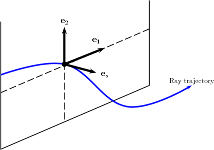
At any point of the ray one can introduce a set of three orthogonal unit vectors,
known as the polarization vectors;
naturally,
the first polarization vector is
.
At any point of the ray one can introduce a set of three orthogonal unit vectors,
known as the polarization vectors;
naturally,
the first polarization vector is
![]() ;
the other two polarization vectors,
which are going to be represented as
;
the other two polarization vectors,
which are going to be represented as
![]() and
and
![]() ,
are within the plane perpendicular to
,
are within the plane perpendicular to
![]() (see Fig.3.2).
(see Fig.3.2).
The vectors
![]() and
and
![]() define the possible orientations of
define the possible orientations of
![]() and
and
![]() at any
coordinate
at any
coordinate ![]() of the ray:
of the ray:
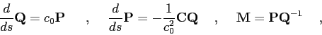
Besides matrices
![]() and
and
![]() the Gaussian beam approximation involves two more matrices,
called
the Gaussian beam approximation involves two more matrices,
called
![]() and
and
![]() ;
all four matrices are related through the following relationships:
;
all four matrices are related through the following relationships:
Orlando Camargo Rodríguez 2012-06-21
![\begin{displaymath}
P(s,\mbox{$\mathbf{n}$}) = \frac {1}{4\pi} \sqrt{ \frac {c_0...
...hbf{n}$}\cdot\mbox{$\mathbf{n}$} \right) \right] \right\} ,
\end{displaymath}](img98.png)
![\includegraphics[height=80mm]{gaussbeam02}](img109.png)
![\begin{displaymath}
\mbox{$\mathbf{P}$}=
\left[
\begin{array}{cc}
p_{11} & p_{12} \\
p_{21} & p_{22}
\end{array} \right]
,
\end{displaymath}](img119.png)
![\begin{displaymath}
\mbox{$\mathbf{Q}$}=
\left[
\begin{array}{cc}
q_{11} & q_{12} \\
q_{21} & q_{22}
\end{array} \right]
,
\end{displaymath}](img120.png)
![\begin{displaymath}
\mbox{$\mathbf{C}$}=
\left[
\begin{array}{cc}
C_{11} & C_{12} \\
C_{21} & C_{22}
\end{array} \right] ,
\end{displaymath}](img121.png)