Solving the transport equation

The solution of the Eikonal equation allows to calculate the Jacobian $J$, between the usual set of cartesian coordinates $(x,y,z)$ and a particular set of ray coordinates $(s,\alpha_1,\alpha_2)$, where $s$ stands for the ray arclenght and $\alpha_{1,2}$ stand for some sort of auxiliary ray angles. In general, $J$ represents the cross section of a ray tube propagating from the source to the receiver. Let us define $\mbox{$\mathbf{e}$}_s$ as the unitary vector tangent to the ray:

$$\mbox{$\mathbf{e}$}_s = \left[ \begin{array}{c} dx/ds \\ dy/ds \\ dz/ds \end{array} \right] .$$ (2.26)

Therefore, the first term in the transport equation, combined with the Eikonal equation, can be rewritten as

$$\mbox{\boldmath$\nabla$}A\cdot\mbox{\boldmath$\nabla$}\tau =... ... {1}{c}\mbox{$\mathbf{e}$}_s = \frac {1}{c}\frac{dA}{ds} .$$

As for the second term, let us notice that the analytical properties of the Jacobian[3] allow to write that

$$\mbox{\boldmath$\nabla$}^2\tau = \mbox{\boldmath$\nabla$}\cdo... ...\tau = \frac {1}{J}\frac{d}{ds}\left( \frac {J}{c} \right) .$$

The previous expressions transform the transport equation into

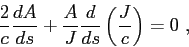$$\frac {2}{c} \frac{dA}{ds} + \frac {A}{J}\frac{d}{ds}\left( \frac {J}{c} \right) = 0 ,$$ (2.27)

which can be easily integrated to provide the result

$$A = \frac{A_0}{ \sqrt{J/c(s)} } ,$$

where $A_0$ stands for a constant, which depends of the type of acoustic source. The solution to the wave equation can then be written as

$$P(\mbox{$\mathbf{r}$},\omega ) = A_0\sqrt{ \frac {c(s)}{J} }\; e^{-i\omega \tau} .$$

In the proximity of a point source one can identify the ray coordinates $(s,\alpha_1,\alpha_2)$ with the spherical coordinates $(s,\theta,\phi)$, centered at the source position (see Fig.2.2); therefore, it can be written that

$$c(s) \approx c(0) \hskip5mm \makebox{and} \hskip5mm J \approx s^2\cos\theta(0) ,$$

with $\theta(0)$ standing for the launching angle. On the oher side, close to the source, the acoustic field can be approximated as a spherical wave, which implies that

$$A_0\sqrt{ \frac {c(0)}{s^2\cos\theta(0)} }\; e^{-i\omega s/c(0)} = \frac {1}{4\pi s} \; e^{-i\omega s/c(0)} ;$$

it follows from this relationship that

$$A_0 = \frac{1}{ 4\pi} \sqrt{\frac{\cos\theta(0)}{c(0)}} .$$

Figure 2.2: Ray coordinates in the proximity to the source.

The classical solution can then be written explicitely as

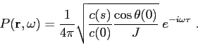$$P(\mbox{$\mathbf{r}$},\omega ) = \frac {1}{4\pi}\sqrt{ \frac {c(s)}{c(0)} \frac {\cos\theta(0)}{J} }\; e^{-i\omega \tau} .$$ (2.28)

Unfortunately, the classical solution based on the Jacobian suffers from a serious drawback. Each time a ray tube narrows into a single point the Jacobian becomes zero (the points at which $J = 0$ are called caustics), and the acoustic field exhibits a singularity at such point. Removing such singularities from the solution can be achieved by substituting the classical solution with the solution based on Gaussian beams.