Let us consider an environment with the following set of conditions:
(i.e., there is no dependence on the second component of
 ,
and indexing is being omitted by obvious reasons) and
,
and indexing is being omitted by obvious reasons) and
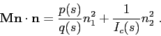
so the matrix contains only diagonal elements,
and we introduced the notation
so det
 .
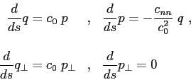
It follows from the system given by Eq.(3.2) that
.
It follows from the system given by Eq.(3.2) that
and
where  and
and
 .
The solution of the last equation is trivial and corresponds to
.
The solution of the last equation is trivial and corresponds to
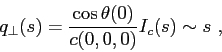
It follows further that
where
Recalling
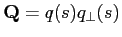
as two-dimensional vector one gets that
 |
(3.6) |
In the case of a point source it follows that
which indicates that the parameter is proportional to the ray path.
Orlando Camargo Rodríguez
2012-06-21
![\begin{displaymath}
\mbox{$\mathbf{C}$}=
\left[
\begin{array}{cc}
c_{nn} & 0 \\
0 & 0
\end{array} \right]
\end{displaymath}](img134.png)
![\begin{displaymath}
\mbox{$\mathbf{Q}$}(s) =
\left[
\begin{array}{cc}
q(s) & 0 \\
0 & q_{\perp} (s)
\end{array} \right]
\end{displaymath}](img135.png)