Calculating the derivatives of sound speed is one (among many) of the most important tasks for an accurate
calculation of ray coordinates,
and further calculations of ray influence at a given point of the array.
To this end TRACEO relies on three different types of piecewise interpolation:
- Linear interpolation: the method is trivial and does not require explanation;
it is applied every time the interpolation point is located between the first or last pair of tabulated coordinates;
being linear, no second derivative is calculated.
- Parabolic interpolation: the method implemented is called barycentric parabolic interpolation;
it is applied every time the interpolating point is located between the first or last three tabulated coordinates.
The method can be described as follows:
let us consider a set of three points
 ,
,  and
and  ,
and the corresponding function values
,
and the corresponding function values  ,
,  and
and  .
At a given point
.
At a given point  (see Fig.5.2) the interpolant can be written as
 |
(5.10) |
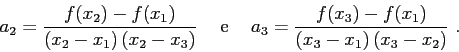
It follows from this expression that
The approximations to the derivatives become
and
Figure 5.2:
1D Barycentric parabolic interpolation.
|
![\includegraphics[width=80mm]{parinterp}](img246.png) |
- Cubic interpolation: the method of interpolation
(not surprisingly called barycentric cubic interpolation)
is analogous to the previous one,
but using four points instead of three.
Cubic interpolation is applied when the interpolation point is surrounded by four points
(two points back and two points forward).
One of the advantages of the barycentric interpolators is that they can be easily extended to
handle different numbers of points,
or to handle interpolation and calculation of derivatives at higher dimensions.
For instance,
the explicit form ot the 2D barycentric parabolic interpolator corresponds to
 |
(5.11) |
(see Fig.5.3) where the coefficients can be calculated as:
Figure 5.3:
2D Barycentric parabolic interpolation.
|
![\includegraphics[width=80mm]{biparinterp}](img251.png) |
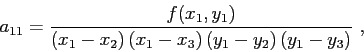
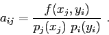
Using the notation
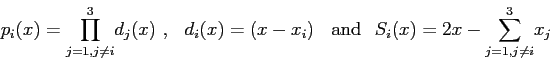 |
(5.12) |
one can write the 2D interpolator compactly as
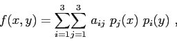 |
(5.13) |
with the coefficients given by
The explicit expressions for the partial derivatives correspond to
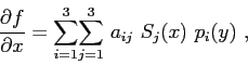 |
(5.14) |
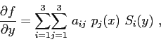 |
(5.15) |
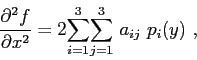 |
(5.16) |
 |
(5.17) |
and
 |
(5.18) |
Orlando Camargo Rodríguez
2012-06-21