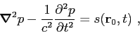
The starting point for the discussion of the ray tracing is given by the acoustic wave equation,
which in the case of a watercolumn with a constant density can be written as
 |
(2.1) |
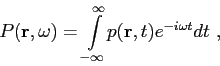
where
 stands for the pressure of the acoustic wave,
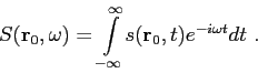
 represents the signal transmitted by the acoustic source,
 represents the source position and
 represents the nabla differential operator.
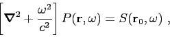
Applying a Fourier transform to both sides of Eq.(2.1) one can obtain
the so called Helmholtz equation:
represents the nabla differential operator.
Applying a Fourier transform to both sides of Eq.(2.1) one can obtain
the so called Helmholtz equation:
 |
(2.2) |
where
and
Let's consider a plane wave-like approximation to the solution of Eq.(2.2)
and write that [4]
 |
(2.3) |
where  represents a slowly changing wave amplitude,
and
represents a slowly changing wave amplitude,
and  stands for a rapidly evolving phase;
the surfaces with constant represent the wavefronts;
analogously,
the surfaces with constant
stands for a rapidly evolving phase;
the surfaces with constant represent the wavefronts;
analogously,
the surfaces with constant  are called timefronts.
By placing Eq.(2.3) into the homogeneous form of Eq.(2.2),
considering the high frequency approximation
are called timefronts.
By placing Eq.(2.3) into the homogeneous form of Eq.(2.2),
considering the high frequency approximation
(where  ) and separating the real and imaginary terms of the equation,
one can obtain the Eikonal equation:
) and separating the real and imaginary terms of the equation,
one can obtain the Eikonal equation:
 |
(2.4) |
and the transport equation:
 |
(2.5) |
The following sections will describe the solution of Eqs.(2.4)-(2.5).
Orlando Camargo Rodríguez
2012-06-21