Deep water

A classical ray tracing test consists in the calculations of ray coordinates for a Munk profile and flat boundaries, with a source at 1000 m depth and a propagating range of 100 km (see [11]). In order to show TRACEO's ability to deal simultaneously with refraction and reflection over range the test was extended by including variable boundaries: on top an idealized sinusoidal surface (a feature which can be of interest for the study of scattering problems), while on bottom the variable bathymetry was given by a Gaussian sea mountain. In a second test the model's stability is further demonstrated, by replacing the Munk profile with an idealization of a Munk field. Both ray traces require the calculation of ray coordinates; in every case TRACEO produces a mat file, called 'rco.mat', which contains a vector of launching angles, and a set of matrices called 'ray1', 'ray2',..., one per each launching angle. Ray information is stored in each matrix as follows:

Row 1:	ray range $r$;
Row 2:	ray range $z$.

The Munk profile used in the first test can be seen in Fig.7.1. The ray plot shown in Fig.7.2 is produced by running the command

» varbounds_profile.m

inside Matlab's prompt. As shown by the figure ray boundary reflections and refraction are properly handled by the model.

Figure 7.1:Canonical Munk profile.	Figure 7.2: TRACEO ray trace.

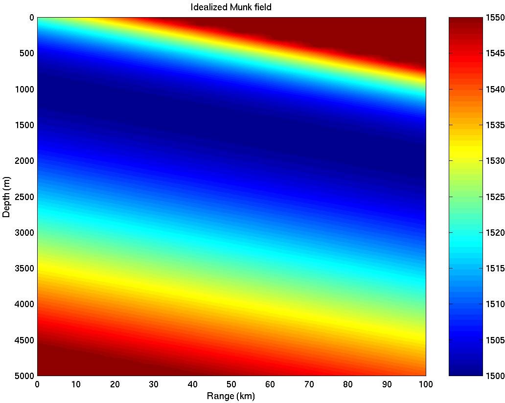
The second example idealizes a waveguide with the same boundaries as the first example, but considers a sequence of Munk profiles, with the axis channel depth deepening from 1000 m to 2000 m, when going from 0 to 100 km (see Fig.7.3). Such field reproduces approximately, on a small scale, the variation of sound speed when moving from the poles to the equator. The resulting ray trace, shown in Fig.7.4, is produced by running the command

» varbounds_field.m

The figure confirms the expected channeling of ray energy along range, from shallow to deep waters, which is induced by the deepening of the deep sound channel. As in the first example, TRACEO keeps a proper handling of boundary reflections.

Figure 7.3: Idealized Munk field.	Figure 7.4: TRACEO ray trace