Shallow water

The shallow water case corresponds to a Pekeris waveguide with flat boundaries, as shown in Fig.7.5. Running the command

» pekeris_rco.m

produces Fig.7.6, which at a first glance does not look particularly interesting; however, the ray pattern changes drastically if the boundary types are changed from 'V' (for the surface) and 'E' (for the bottom) to 'A'; in such case, running the previous command produces now the ray trace shown in Fig.7.7, which predicts the lack of wave interference, previously induced by ray reflections. Additionally, other patterns will be generated by changing to 'A' only one of the two boundary types.

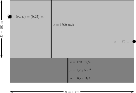Figure 7.5: The flat Pekeris waveguide (vacuum on top).

Figure 7.6: Pekeris waveguide: ray coordinates (top vacuum, bottom elastic).

Figure 7.7: Pekeris waveguide: ray coordinates (top and bottom absorbers).

If the output option 'RCO' is changed to 'ARI' running the command

» pekeris_rco.m

produces now a mat file, called 'ari.mat'; again, ray information is stored in matrices 'ray1', 'ray2',..., but now each matrix contains the following information:

Row 1:	ray range $r$;
Row 2:	ray depth $z$;
Row 3:	ray travel time $\tau$;
Row 4:	real part of ray amplitude Re$(a)$;
Row 5:	imaginary part of ray amplitude Im$(a)$.

Eigenray calculations shown in Fig.7.8) are produced by running the command

» pekeris_eig.m

with the output options 'ERF' and 'EPR'. Eigenray calculations produce a 'eig.mat' mat file, with information stored as in the 'ari.mat' output file. The second case uses five times more launching angles than the first, and still so the number of eigenrays is smaller. At a first glance eigenray search by proximity seems inefficient.

Figure 7.8: Pekeris waveguide: eigenrays calculated by Regula Falsi (top) and by proximity (bottom).

The advantage of eigenray search by proximity over search by regula falsi is revealed by running the command

» pekeris_wedge_eig.m

which produces Fig.7.9; in fact, eigenray search in this case is only possible with the 'EPR' option.

Figure 7.9: Pekeris waveguide with a wedge: eigenrays calculated by proximity.

A demonstration of TRACEO's arrival calculations is shown in Fig.7.8), which is produced by running the command

» pekeris_aad.m

with the output option 'ADR'. Arrival calculations produce a mat file, called 'aad.mat'; arrival information is stored in vectors 'aad1', 'aad2',..., one per each eigenray; each vector contains the following information:

Element 1:	hydrophone range $r_h$;
Element 2:	hydrophone depth $z_h$;
Element 3:	eigenray travel time $\tau$;
Element 4:	real part of eigenray amplitude Re$(a)$;
Element 5:	imaginary part of eigenray amplitude Im$(a)$.

Arrival predictions shown in Fig.7.10 indicate a system of arrivals, clustered in groups of four arrivals; as expected from the symmetry between the source and the receiver central arrivals overlap, transforming the quadruplet groups in groups of triplets.

Figure 7.10: Pekeris waveguide: travel times and amplitudes calculated by Regula Falsi.

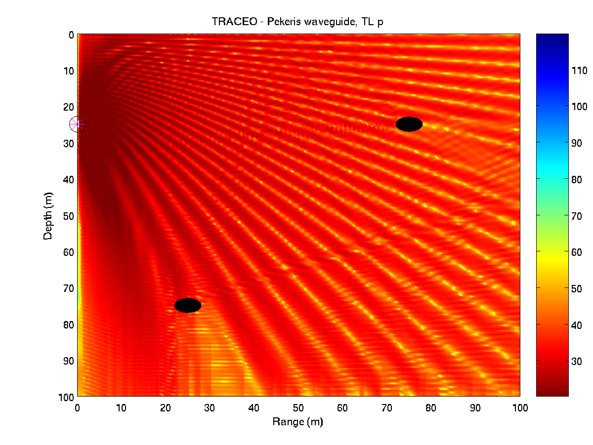
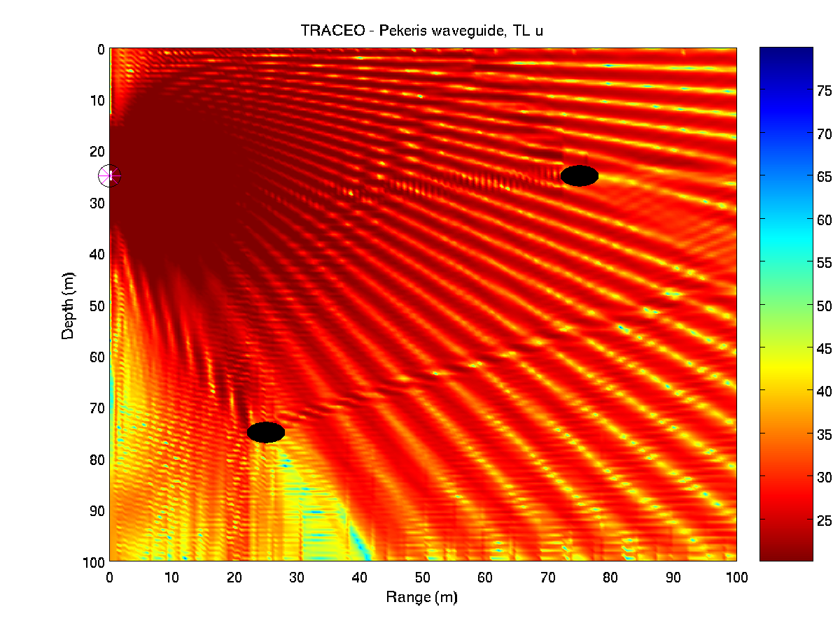
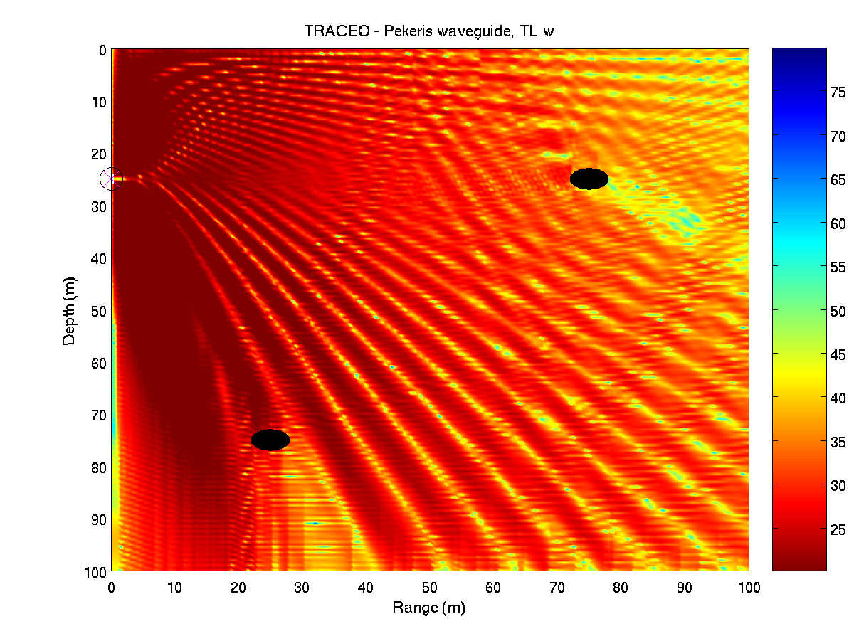
Transmission loss calculations with two ellipsoidal objects, at the positions $[25,75]$ m and $[75,25]$ m, are shown in Fig.7.11; the figure is produced by running the command

» pekeris_pav2o.m

with the output option 'PAV'. Acoustic pressure and particle velocity calculations produce a mat file, called 'pav.mat'; for a rectangular array the information is stored in matrices 'rp', 'ip', 'ru', 'iu' and 'rw', 'iw', which contain the real and imaginary parts of $p$, $u$ and $w$, respectively. For a linear array the information is stored in vectors 'p', 'u' and 'w', each containing the following information:

Row 1:	real part;
Row 2:	imaginary part.

In both cases the coordinates of the array are stored, together with the requested quantities. Fig.7.11 reveals a partial blocking of the acoustic field in the waveguide, with clear differences in the interference patterns of $p$, $u$ and $w$. Although no clear diffraction is visible around the objects all cases indicate that the presence of the objects induces a significant redistribution of wave energy.

Figure 7.11: Pekeris waveguide: transmission loss for pressure (top), horizontal component of particle velocity (middle), and vertical component of particle velocity (bottom).