Deep water ray tracing

A classical test for ray tracing consists in deep water ray calculations with a Munk profile and flat boundaries, with a source at 1000 m depth and 100 km range (see [4]). In order to test Trace stability when dealing simultaneously with refraction and reflection over range the classical test was expanded here by including variable boundaries: on top an idealized sinusoidal surface (a feature which can be of interest for the study of scattering problems), while on bottom ray propagation should be affected by the variable bathymetry of a Gaussian sea mountain. In a second test the stability of Trace was further tested by replacing the profile with an idealization of a Munk field.

The Munk profile used in the first test can be seen in Fig.1. The M-file readari.m was used to read the *.ray OUTFIL produced by Trace, and to produce the ray plot shown in Fig.2. As seen in the figure boundary reflections and ray refraction are properly handled by the model.

Figure 1: Munk sound speed profile.
Figure 2: Ray trace with the previous Munk profile and variable boundaries.

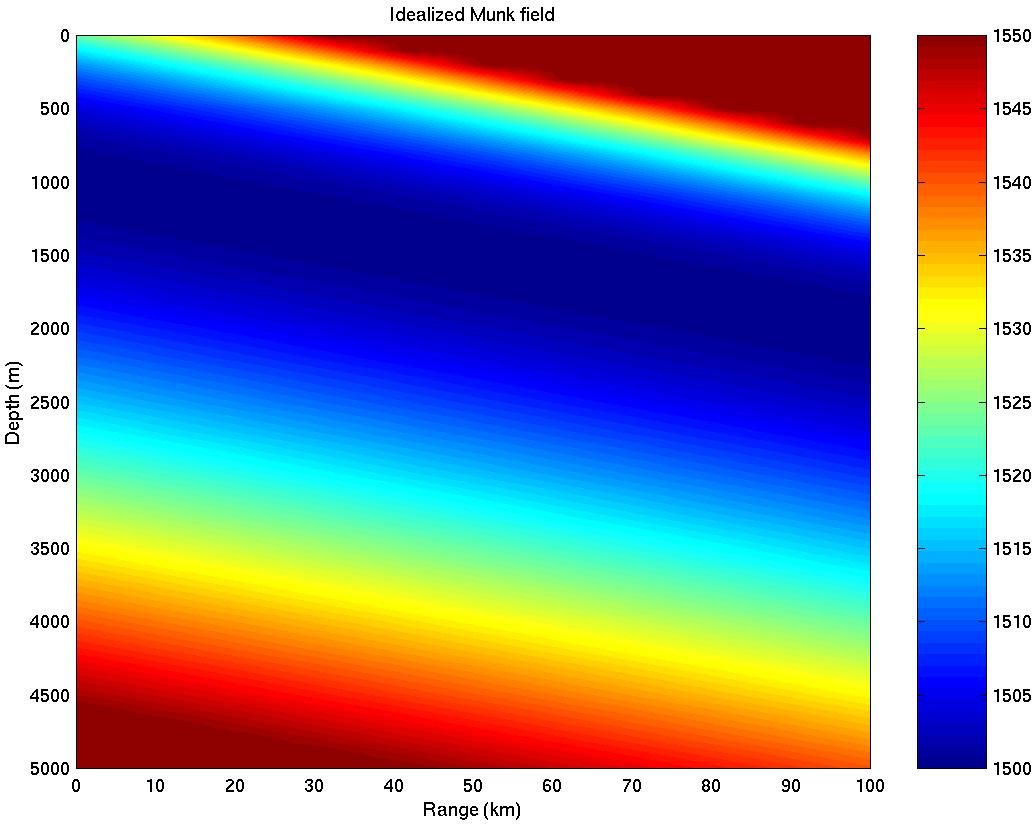
The idealized Munk field used in the second ray tracing test was composed of a sequence of Munk profiles, with the axis channel depth deepening from 1000 m to 2000 m between 0 and 100 km (see3). The field reproduces approximately at a small scale the behaviour of sound speed between the poles and the equator. The resulting ray trace is shown in Fig.4 and shows the expected trapping of ray energy due to refraction around the deep sound channel. Moreover, boundary reflections remain properly handled by Trace.

Figure 3: Idealized Munk sound speed field.
Figure 4: Ray trace with the previous Munk field variable boundaries.