Shallow water isovelocity calculations

In order to show in detail the different calculations that can be performed with Trace&Traceo let us consider the simple case of an isovelocity waveguide, as shown in Fig.5.

Figure 5: The baseline environment for isovelocity calculations (vacuum on top).

The WAVFIL containing the description of the environment (and named isowaveguide.wav ) looks like follows:

'TRACE - isovelocity waveguide'
------------------------------------------------
1.000000
0.000000
25.000000
1500.000000
500.000000
'GMB'
51
-20.000000 20.000000
------------------------------------------------
'V'
'2P'
2
0.000000e+00 0.000000
1.000000e+03 0.000000
------------------------------------------------
'c(z,z)'
'ISOV'
2
   0.000000 1500.000000
100.000000 1500.000000
------------------------------------------------
'H'
'2P'
'W'
1700.000000 1.700000 7.000000e-01
2
0.000000e+00 100.000000
1.000000e+03 100.000000
------------------------------------------------
'RCO'
'UAS'
1 1
1.000000e+03 
1.000000e+02 
75.000000 1.000000

As shown by the option 'RCO' the WAVFIL indicates Trace to perform the calculation (only) of ray coordinates, making irrelevant the shape of the array (which contain only a single element), and the position of the hydrophone where eigenrays are to be calculated. Running 'runtrace isowaveguide' produces two output files, the first is the LOGFIL (named isowaveguide.log), which is written no matter what the output option is and looks like follows:

  TRACE ray tracing program
  INPUT: waveguide file...
 TRACE - isovelocity waveguide                               
 OUTPUT: RAYFIL with ray coordinates...
 Boundary attenuation units: (dB/wavelength)...
 done.
  
 CPU time:  0.465928972 seconds

and a RAYFIL (named isowaveguide.ray), which can be read with the M-file readrco.m and produces Fig.6.

Changing 'RCO' to 'ARI' and running the program takes slightly longer. This time the RAYFIL contains detailed information regarding every ray calculated by the model, specifically:

• travel time, arrival amplitude and decay due to reflections;
• ray coordinates and sound speed along the ray;
• reflection coefficients;
• reflection points;
• refraction points;
• emission and arrival angles;
• phase shifts due to frequency, caustics and reflections.

Reading the RAYFIL with the M-file readari.m produces again Fig.6.

Figure 6: Preliminary ray trace for the isovelocity environment.

Changing 'ARI' to 'EIG' produces a RAYFIL, which contains only the eigenrays that connect the source and the receiver¹. Reading the RAYFIL with the M-file readari.m produces Fig.7.

Figure 7: Eigenrays for the isovelocity environment.

A present disadvantage of eigenray search resides in the fact that it can be performed at a single hydrophone only (the one located at the zeig depth). If required, travel time and amplitude data can be calculated at the receiving array by changing 'EIG' to 'AAD' and defining an array with the desired configuration. For simplicity the array chosen here coincides with the hydrophone used for eigenray calculations, so the Output Block looks like:

----------------------------------
'AAD'
'UAS'
1 1
1.000000e+03 
7.500000e+01 
75.000000 1.000000

(the last line, with the parameters zeig and miss is ignored by the program). Running the program produces an ARRFIL, which can be read with the M-file readaad.m and produces Fig.8. As expected from the symmetry between the source and the receiver the figure shows a system of quadruplet groups, with central arrivals overlapping in arrival time, producing triplets.

Figure 8: Arrivals calculated at the position of the hydrophone.

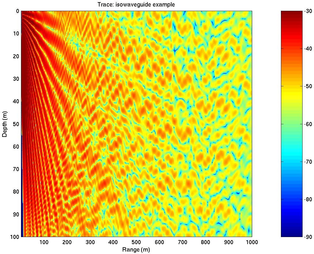
Acoustic pressure can be calculated at the array changing 'AAD' to 'CPR', which can be used in Matched Field Processing. Running the program produces an output file (named in this case as 'isowaveguide.press'), which can be read with the M-file readpress.m. However, many acousticians prefer to look at transmission loss, which can be calculated changing 'CPR' to 'CTL'. The output file (named in this case as 'isowaveguide.tl'), can be read with the M-file readtl.m (see Fig.9). In order to obtain a detailed structure of interference the calculations were performed with an array of 501$\times$501 elements, so the Output Block was looking like:

----------------------------------
'CTL'
'UAS'
501 501
0.000000e+00 2.000000e+00 4.000000e+00 .... 1.000000e+03
0.000000e+00 2.000000e-01  4.000000e-01  .... 1.000000e+02 
75.000000 1.000000

Figure 9: Transmission loss at 500 Hz calculated along a rectangular array of 501$\times$501 receivers.

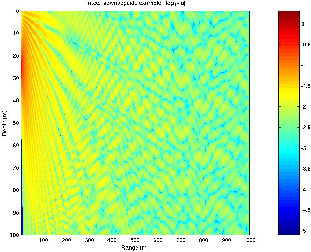
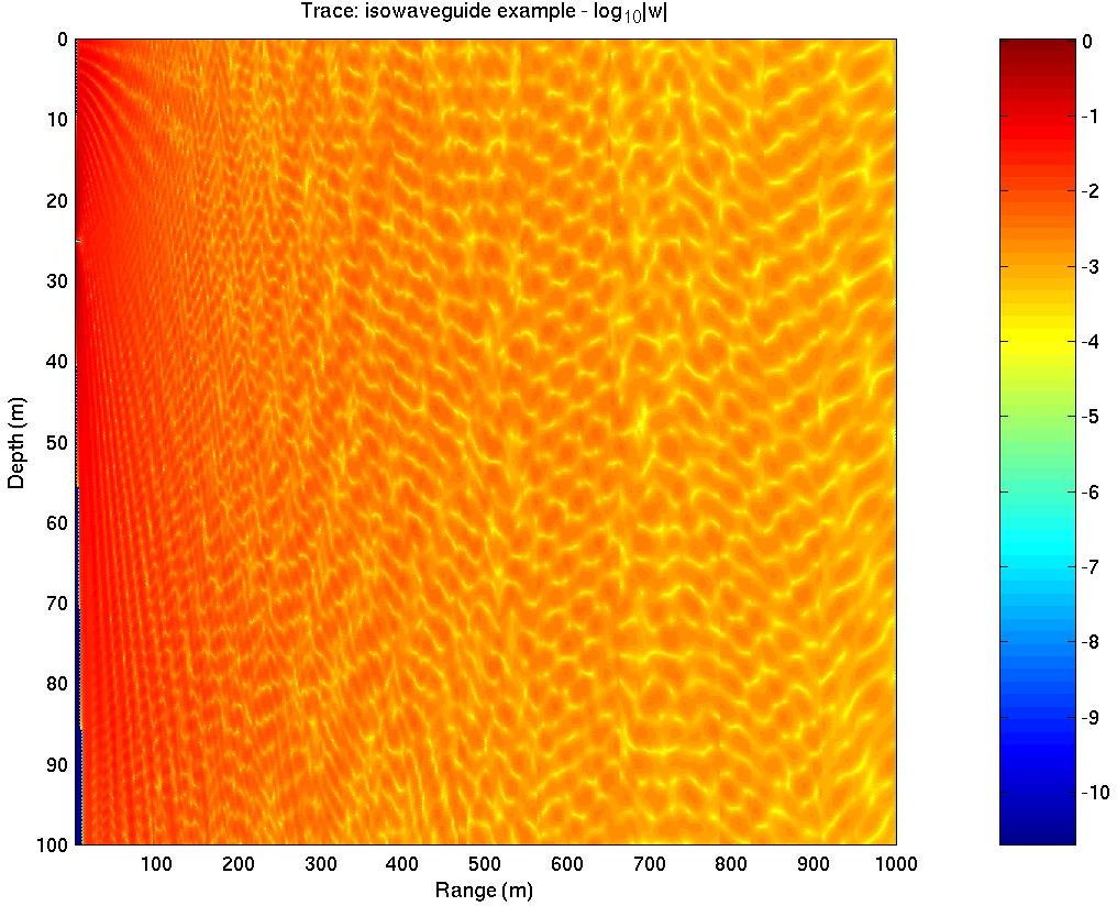
Changing 'CTL' to 'PVL' allows to illustrate the last option used by the programs, which allows to calculate the particle velocity (see Fig.10 and Fig.11). Such calculations are expected to be of interested in the modeling of vector sensor arrays.

Figure 10: Horizontal component of particle velocity at 500 Hz calculated along a rectangular array of 501$\times$501 receivers.
Figure 11: Vertical component of particle velocity at 500 Hz calculated along a rectangular array of 501$\times$501 receivers.