Geometric beams
As shown by numerical calculations the solution of the dynamic equations
(see Eq.(3.8)) with complex values induces the formation of weird artifacts,
which reveal themselves as patterns of self-interference after the ray is reflected on a boundary.
In some cases such interference is unrealistically intense despite the expected exponential decay in
amplitude along the normal direction.
To erradicate such artifacts TRACEO uses the approximation of geometric beams[11,12],
which relies on the following expression for the calculation of the acoustic field:
![\begin{displaymath}
P(s,n) = \phi(s,n) a e^{ -i\left[ \omega \tau(s,n) - \phi_c \right] } ;
\end{displaymath}](img202.png) |
(5.1) |
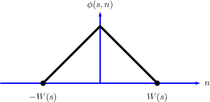
in the above expression  is a hat window (see Fig.5.1),
defined as
is a hat window (see Fig.5.1),
defined as
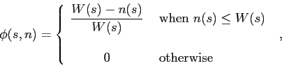 |
(5.2) |
with  representing the beam width:
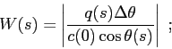 |
(5.3) |
in this expression  stands for the angle step.
Figure 5.1:
Geometric beams: the hat function.
|
|
Moreover,
the dynamic equations are integrated using the initial conditions:
which provide the following expression for the amplitude:
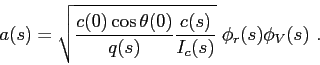 |
(5.4) |
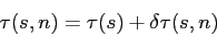
By using real values of  and
and  it becomes necessary to compensate the travel
time along the normal direction;
such compensation can be written as
it becomes necessary to compensate the travel
time along the normal direction;
such compensation can be written as
 |
(5.5) |
where  is the classical travel time (see Eq.(2.9));
the additional term corresponds to
is the classical travel time (see Eq.(2.9));
the additional term corresponds to
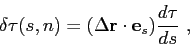 |
(5.6) |
where
with
 and
and
 representing, respectively,
the position of the hydrophone and the position of the given point along the ray.
The total acoustic field is then calculated as a superposition of all ray influences.
representing, respectively,
the position of the hydrophone and the position of the given point along the ray.
The total acoustic field is then calculated as a superposition of all ray influences.
A drawback of the geometric beams is that they are affected by caustics,
as the classical solution,
because of the changes in sign of as the integration proceeds along the ray arclength.
As discussed in [11] the general behaviour of the solution can still be accurate
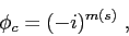
by introducing an amplitude correction  into Eq.(5.1),
which can be written as
into Eq.(5.1),
which can be written as
 |
(5.7) |
where  represents the imaginary unit,
and
represents the imaginary unit,
and  corresponds to the number of times that vanishes in the interval
![$\left[ 0,s \right] $](img220.png) (this function is also known as the KMAH index).
(this function is also known as the KMAH index).
Orlando Camargo Rodríguez
2012-06-21
![\begin{displaymath}
\Delta\mbox{$\mathbf{r}$}= \mbox{$\mathbf{r}$}_h - \mbox{$\m...
...egin{array}{c}
r_h - r(s) \\
z_h - z(s)
\end{array} \right]
\end{displaymath}](img214.png)